Math Functions can be very useful to perform operations on your input data but are also used for comparison and value finding objectives.  These helpful functions allow you to perform such operations as addition, subtraction, finding maximum or minimum values, and more.  In this section, you can find information on the available Math Function and how they can assist you in meeting your Data Diagram design needs.

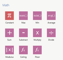
Figure 1:  The Math Functions as displayed in the Functions dialog.

Usage

To insert a Math Function, select Functions in the Side Menu.  You will notice that the Math group displays options that you can choose from.  Below you can find detailed information on each.  For these examples, we will use a database Table as an input data source, and perform our operations on the UnitPrice field.  You can select a Function from the list provided below to navigate to that particular function.

 

 

You will often need to use Constants to define values for your testing that are static. Constants can be a variety of different types such as integer, string, and date and hold the value that you specify.  We'll take an example based upon our sample database Table source.  If we wanted to filter the data set such that only values of UnitPrice greater than 50 are to be included in our output data, we would need to declare a Constant of integer value type and set the value to 50.  Once inserted into the Data Diagram, simply double click on Function object to access the Properties dialog.

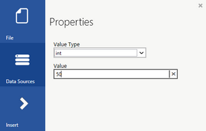
Figure 2:  Setting the Constant type and value in the Properties Dialog.

 

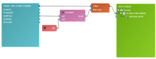
Figure 3:  A Constant is used as an input parameter for a function.

This Function can be useful when you are in need of comparing two or more values and returning the maximum value of the two.  As an example, we only want to  display prices in our output as 20 and above.  We will use the Max() function to test UnitPrice against a Constant that is set to 20.  Here you will see that for every UnitPrice, whichever value is greater, 20 or the UnitPrice value, will be displayed.

 

By default, the Max() Function has two input value connectors.  You can add additional parameters by right clicking and selecting Add Parameter from the Application Bar. Below you can find a sample diagram and it's resulting output.

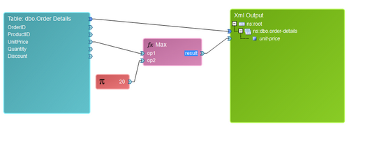
Figure 4:  A Max() Function is used to compare values.

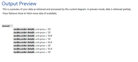
Figure 5:  The output reveals the function returns either a 20 or larger value.

 

This Function can be useful when you are in need of comparing two or more values and returning the minimum value of the two.  As an example, we only want to  display prices in our output as 20 and below.  We will use the Min() function to test UnitPrice against a Constant that is set to 20.  Here you will see that for every UnitPrice, whichever value is less, 20 or the UnitPrice value, will be displayed.

 

By default, the Min() Function has two input value connectors.  You can add additional parameters by right clicking and selecting Add Parameter from the Application Bar. Below you can find a sample diagram and it's resulting output.

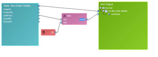
Figure 6:  A Min() Function is used to compare values.

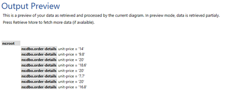
Figure 7:  The output reveals the function returns either a 20 or a lesser value.

The Average function is useful when you would like to calculate the average of two or more input values.  As an example, let's imagine that the previous two years, a  standard discount has been given of 2 and 3 dollars.  Given that each order has its own discount value, we can compute an average discount, per product, to determine what the average discount has been per order.  In this example, we'll use Constants to portray the previous two year discount values.

By default, the Average Function has two input value connectors.  You can add additional parameters by right clicking and selecting Add Parameter from the Application Bar.  Here we have done so to add a third parameter. Below you can find a sample diagram and it's resulting output.

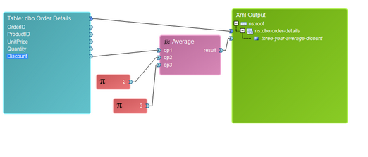
Figure 8:  An Average Function is used to compute the average of 2 constants and a table value.

 

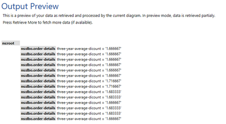
Figure 9:  The output preview reveals a 3 year average discount per order.

The Sum function is useful when you would like to find the Sum of two or more values.  As an example, we may know that for every order placed, there is a standard processing fee of 2 dollars.  This would mean that we would need to include a sum of both the UnitPrice value and a constant with value of 2 to get the finalized UnitPrice which includes the standard processing fee.

 

By default, the Sum Function has two input value connectors.  You can add additional parameters by right clicking and selecting Add Parameter from the Application Bar. Below you can find a sample diagram and it's resulting output.

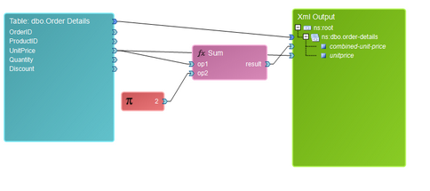
Figure 10:  The Sum Function is used to sum both a table value and a constant.

 

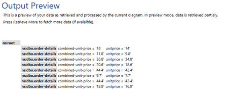
Figure 11: The output preview displays the Sum Function results.

The Subtract function is useful for when you would like to subtract two or more values.  As an example, we want to find the final price after applying a discount.  We use a Subtract function to first specify the UnitPrice field as a parameter and then the Discount field as a parameter.  The result will yield a final price of the order after subtracting the discount.

 

By default, the Subtract Function has two input value connectors.  You can add additional parameters by right clicking and selecting Add Parameter from the Application Bar. Below you can find a sample diagram and it's resulting output.

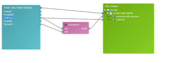
Figure 12:  The Subtract Function is used to subtract one table field from another.

 

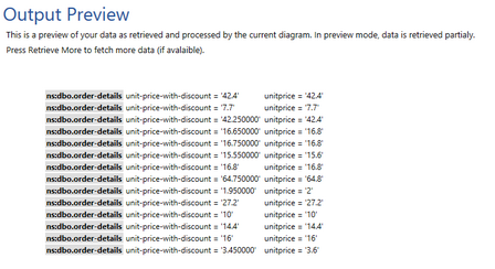
Figure 13:  The output preview screen displays adjusted unit prices with discount applied.

The Multiply function is used to find the product of two values.  As an example, if you wanted to find the total order amount, you would be in need of multiplying the UnitPrice field by the Quantity field to obtain the total order amount.

 

By default, the Multiply Function has two input value connectors.  You can add additional parameters by right clicking and selecting Add Parameter from the Application Bar. Below you can find a sample diagram and it's resulting output.

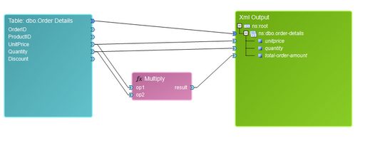
Figure 14:  The Multiply Function is used to find the product of two values.

 

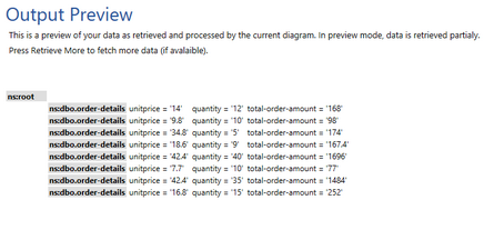
Figure 15:  The output preview reveals the total order amount as computed by the multiply function.

The Divide function is used to find the divide one data value by another.  An example of such usage would be if, for shipping purposes, every order quantity had to be divided by 2 and displayed in the output XML for printing purposes.  When inserting a Divide function, you can specify both the dividend and the divisor.  In our example, we have specified our dividend to be the Quantity field and the divisor to be a Constant assigned the value of 2. Below you can find the example diagram demonstrating this, as well as the corresponding output data.

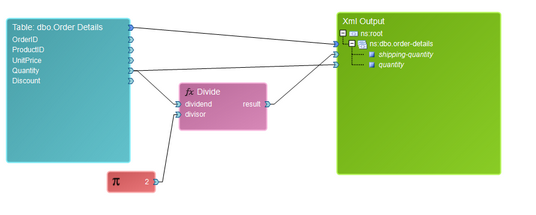
Figure 16:  The Divide Function is used to half the quantity for shipping purposes.

 

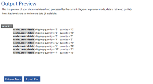
Figure 17:  The results of the Divide Function yield halved values for shipping quantities.

The Modulus function can be useful in examples where any negative value must be returned as a positive value.  An example of such usage is if we incurred a penalty which required a 10 dollar payout per UnitPrice for every order placed.  In some cases we may see that the overall UnitPrice may dip below zero as a negative number.  To also obtain just the value as a positive figure, we will use the Modulus function.  The Modulus function simply has one input Data Connector where you will include the value to use. In this example, we've subtracted 10 first, and with the result, used the Modulus function.

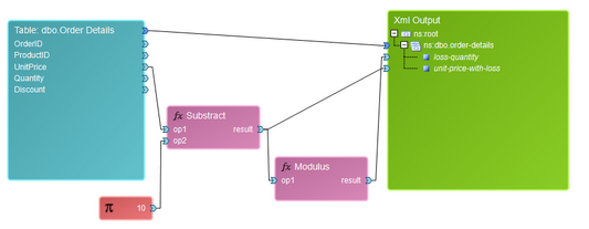
Figure 18:  The Modulus Function is used to find the positive value of the result.

 

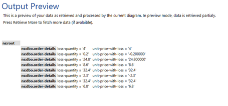
Figure 19:  The results yield that for any negative values, the Modulus Function returns a positive value.

The Ceiling function can be useful if you are looking to obtain the smallest following integer in relation to an input value.  As an example, if we are looking to obtain the next integer price point in relation to our UnitPrice per order, we can use the Ceiling Function to find the smallest following integer.  This function, when inserted, only possesses one input Data Connector.  For this example, we will use the UnitPrice field from our table with our Ceiling Function.

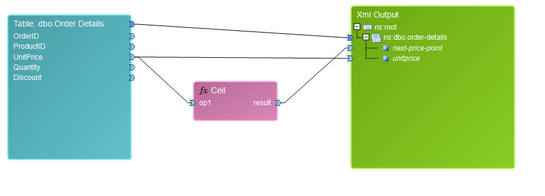
Figure 20:  The Ceiling Function is used in a diagram to return the smallest following integer.

 

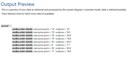
Figure 21:  The Ceiling Function results yield the next price point values.

The Floor function can be useful if you are looking to obtain the largest previous integer in relation to an input value.  As an example, if we are looking to obtain the  previous integer price point in relation to our UnitPrice per order, we can use the Floor Function to find the largest previous integer.  This function, when inserted, only possesses one input Data Connector.  For this example, we will use the UnitPrice field from our table with our Floor Function.

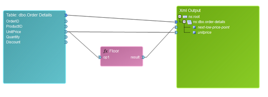
Figure 22:  The Floor Function is used to return the largest previous integer value.

 

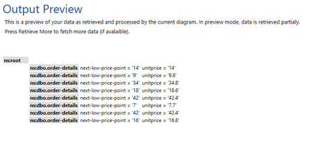
Figure 23:  The output preview displays the largest previous integer as provided by the Floor Function.